
Photo by Aksonsat Uanthoeng from Pexels
If you run OpenAI chat completions in production, you already know that the number you see in a single curl timer is not the number your users in São Paulo, Mumbai, or Frankfurt experience. Latency is regional, it shifts with token count, and it changes throughout the day. The moment you start sending custom token sets, longer system prompts, structured output schemas, or few-shot examples, the variance widens even further. This article breaks down the regional patterns we observe across OpenAI chat endpoints and gives you a practical framework for measuring them with your own payloads.
TL;DR
- OpenAI chat completion latency varies significantly across regions; US-East typically sees the lowest TTFB while Asia-Pacific and South America can add 200–600 ms of network overhead alone.
- Custom token sets (longer prompts, structured outputs) amplify regional differences because processing time scales with input tokens and the network round-trip compounds on top.
- Measuring with a fixed, default prompt hides real-world performance, you need probes that mirror your actual payloads.
- Time-to-first-byte (TTFB) and time-to-first-token (TTFT) are the two metrics that matter most for user-perceived speed in streaming scenarios.
- Observinio probes from 21 regions let you track these patterns daily without building custom infrastructure.
Why default benchmarks lie about your latency

Most public latency benchmarks for OpenAI endpoints use a minimal payload: a short system message, a one-line user prompt, and max_tokens set to something small like 50 or 100. That is useful for comparing models head-to-head, but it tells you almost nothing about what your production traffic actually experiences.
Consider a typical RAG-powered chat feature. Your system prompt alone might be 800–1,200 tokens. You append retrieved context chunks, another 1,500–3,000 tokens. The user's question adds 20–80 tokens. You request 500–1,000 tokens of output. That is a fundamentally different workload from a 30-token "Hello, how are you?" probe.
When you multiply that heavier payload by regional network distance, the differences become stark. A request from us-east-1 to OpenAI's US-based inference cluster might complete its prefill in 400 ms. The same request from ap-southeast-1 (Singapore) adds roughly 180–250 ms of pure network round-trip before the model even starts processing. For streaming responses, that delay lands directly on TTFT, the metric your users feel most acutely.
The compounding effect of token count on regional variance
Latency for chat completions has two main components:
- Prefill time, proportional to input token count. The model processes your entire prompt before generating the first output token.
- Decode time, proportional to output token count. Each subsequent token is generated sequentially (or in speculative batches).
This is why you cannot simply take a US-based benchmark and add a flat "network penalty" for other regions. The ratio shifts depending on your payload size.
Mapping the regional landscape

OpenAI's inference infrastructure is concentrated in the United States, with Azure regions handling much of the compute. This geographic reality creates predictable latency tiers for chat completions:
Tier 1, Lowest latency (< 50 ms network overhead)
- US East (Virginia, Ohio)
- US West (Oregon, California)
- Canada Central (Montreal)
Tier 2, Moderate latency (50–150 ms network overhead)
- Western Europe (Frankfurt, London, Amsterdam, Paris)
- UK South
- Brazil South (São Paulo)
Tier 3, Higher latency (150–300 ms network overhead)
- Asia-Pacific (Singapore, Tokyo, Sydney, Mumbai, Seoul)
- Middle East (UAE, Bahrain)
- Africa (South Africa)
"Responses: mean=4.268s median=2.349s min=1.421s max=21.711s stdev=4.903sChat : mean=1.354s median=1.298s min=0.902s max=2.385s stdev=0.330s Statistical: Store = False." >, Stateful Responses API Much Slower Than Chat Completions
The community data above illustrates how even within a single region, the spread between min and max can be enormous, a 15× difference between the fastest and slowest response. When you layer regional network variance on top of that server-side variance, the tail latencies your global users experience can be dramatically worse than your local testing suggests.
| Region | Network overhead | Typical TTFT |
|---|---|---|
| US East (Virginia) | < 20 ms | 500–800 ms |
| EU West (Frankfurt) | 80–120 ms | 900–1,200 ms |
| Brazil South (São Paulo) | 100–150 ms | 1,000–1,400 ms |
| APAC (Singapore) | 180–250 ms | 1,200–1,600 ms |
| APAC (Sydney) | 200–300 ms | 1,300–1,800 ms |
Designing probes with custom token sets

To get latency data that actually reflects your production experience, your synthetic probes need to mirror your real payloads. Here is a step-by-step approach to building representative probe configurations.
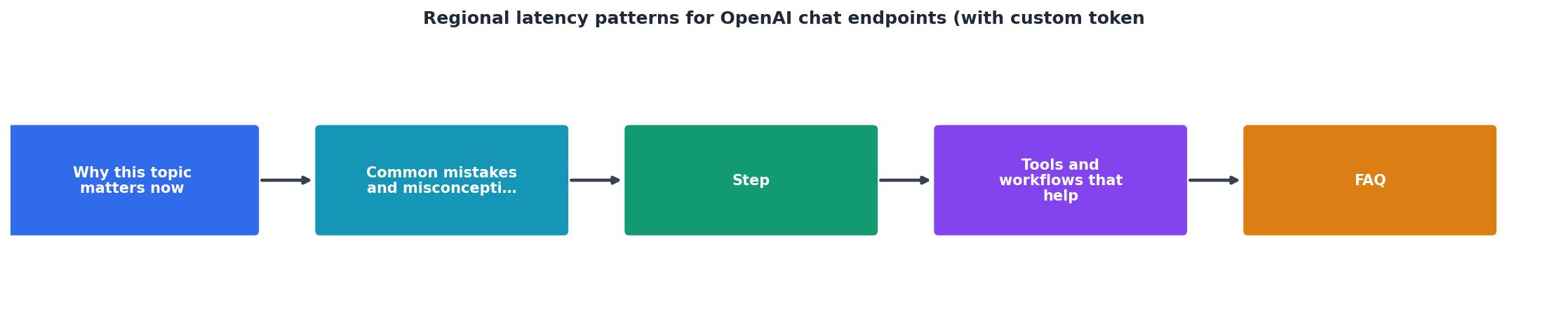
Step 1, Profile your production payloads
Before you configure any probe, sample your actual API calls. Pull a week of logs and compute:
- P50 and P95 input token counts, these define your "typical" and "heavy" payloads.
- P50 and P95 output token counts, determines how long decode runs.
- System prompt length, often fixed or semi-fixed; include it verbatim in your probe.
- Streaming vs. non-streaming ratio, if 90% of your calls stream, your probes should too.
# Example: extract token counts from your OpenAI usage logs
cat openai_requests.jsonl | jq '.usage.prompt_tokens' | sort -n | awk '
  BEGIN {count=0}
  {vals[count++]=$1}
  END {
    printf "P50 input tokens: %d\n", vals[int(count0.5)]
    printf "P95 input tokens: %d\n", vals[int(count0.95)]
  }'
Step 2, Build representative prompt templates
Create two or three probe templates that match your profiled payloads:
- Light probe, matches your P50 input/output. Use this for frequent (every 5–10 minute) checks.
- Heavy probe, matches your P95 input/output. Run this less frequently (every 30–60 minutes) to catch payload-dependent degradation.
- Structured output probe, if you use JSON mode or function calling, include the schema in the probe. Schema validation adds server-side processing time that a plain text probe will not capture.
Step 3, Select target regions
Pick regions where your actual users are concentrated. If you serve a global audience, aim for at least one region per tier from the list above. A minimum viable set for most SaaS products:
- US East (primary)
- EU West (Frankfurt or London)
- Asia-Pacific (Tokyo or Singapore)
- One "canary" region with historically high variance (e.g., Sydney or Mumbai)
Step 4, Establish baselines and set alert thresholds
Run your probes for at least seven days before setting alert thresholds. This captures weekday/weekend patterns and gives you stable P50 and P95 baselines per region. A reasonable starting point for alerts:
- Warning, TTFT exceeds regional P95 baseline by more than 30%.
- Critical, TTFT exceeds regional P95 baseline by more than 100%, or three consecutive probes exceed the warning threshold.
Step 5, Iterate on token sets quarterly
Models change, your prompts evolve, and OpenAI's infrastructure shifts. Re-profile your production payloads every quarter and update your probe templates accordingly. Stale probes give you false confidence.
Practical checklist: regional latency monitoring for OpenAI chat
Use this checklist when setting up or auditing your monitoring:
Your progress is saved automatically in your browser.
What the data tells you (and what it does not)
Regional latency probes with custom token sets answer specific questions very well:
- Is the slowdown regional or global? If Tokyo and Singapore degrade but Frankfurt holds steady, the issue is likely network or routing, not model-side.
- Did a model update change latency characteristics? When OpenAI ships a new model version, your heavy probe will show whether prefill time shifted.
- Are my users in region X getting an acceptable experience? Compare your TTFT probe data against your product's latency SLO.
x-ratelimit-remaining-tokens) for a complete picture.
Key takeaway: Regional latency monitoring with production-representative token sets is the only reliable way to understand what your global users actually experience — default benchmarks from a single location will consistently understate the variance and hide payload-dependent degradation that affects real-world performance.
Time-of-day and day-of-week patterns
OpenAI's infrastructure experiences load patterns that correlate with US business hours. Across multiple weeks of observation, several consistent patterns emerge:
- Lowest latency window: 04:00–08:00 UTC (late night / early morning US time). Prefill times can be 20–35% lower than peak.
- Peak latency window: 15:00–21:00 UTC (US business hours through early evening). This is when queue times on OpenAI's side are highest.
- Weekend effect: Saturday and Sunday show 10–20% lower median latency compared to weekday equivalents, particularly for larger models like GPT-4o.
Frequently Asked Questions
japaneast for Tokyo-based users or westeurope for Frankfurt-based users can cut 100–250 ms off TTFT compared to routing through OpenAI's default US-based endpoints. The tradeoff is managing multiple deployments, potential model availability differences across Azure regions, and higher operational complexity.Start tracking regional patterns today
If you are running OpenAI chat completions for users outside a single US region, you need regional latency data, not aggregated averages from a single probe location. Observinio runs daily probes from 21 global regions, compares results against established baselines, and sends email alerts when degradation is detected. You can review current latency patterns on the status page or configure alerts tailored to the regions and endpoints your product depends on. Visit observinio.com to see how your regions are performing right now.
Additional Resources
- Stateful Responses API Much Slower Than Chat ... - On Chat Completions, GPT-5 (minimal reasoning) is averaging about 5-7 sec for me, even with 50+ message history and almost 100k tokens. On the ...
- High latency for chat completion requests to Azure OpenAI ... - I have a deployment of gpt-4o-mini 2024-07-18 in region swedencentral and started to encounter high latency around 7:38 AM GMT on 2025/11/13. The request ...
- Inconsistent Latency in Asynchronous OpenAI Chat ... - I'm encountering an issue with asynchronous OpenAI API calls where certain requests take significantly longer than others, even though the input ...