
Photo by Niepoddawajsie.pl Luk from Pexels
Retrieval-Augmented Generation (RAG) pipelines have become standard in production AI applications. A user types a question, your system retrieves relevant documents, feeds them to an LLM, and returns an answer. Simple in theory. In practice, each step burns latency: embedding the query, searching your vector store, fetching context, calling the LLM API, streaming tokens back. If any stage stalls, users wait. A 2-second response time feels instant; a 5-second one feels broken.
The core problem: you have a latency budget, and you need to know how to spend it. This article walks through how to measure, allocate, and monitor that budget across your RAG stack, and why regional variance in API latency can blow your timeline before you even know it happened.
- RAG pipelines have multiple latency contributors: embedding, retrieval, LLM inference, and token streaming. Most teams underestimate how much time goes to retrieval.
- A typical SLA might reserve 300 ms for embedding, 150 ms for retrieval, 1200 ms for LLM TTFB (time-to-first-byte), and 100 ms for overhead, totaling 1750 ms.
- Regional latency variance across LLM providers can swing response times by 40–60% without warning; daily probes from 21 regions let you catch degradation early.
- Parallelism (embedding and retrieval in parallel, not serial) can save 30–40% of end-to-end time.
- Monitor TTFB and token streaming rate (tokens/second) separately; they require different optimization strategies.
Key Takeaway
Without a latency budget, RAG pipeline optimization becomes guesswork. By measuring each stage independently and allocating time allocations top-down from your user-facing SLA, you gain visibility into which components truly constrain performance. Regional monitoring from multiple geographic locations reveals provider degradation within hours rather than days, enabling proactive rerouting and informed vendor selection. The difference between a responsive 2-second chat experience and a frustrating 5-second one often comes down to systematic budget tracking and early detection of regional variance.
Why Latency Budgets Matter for RAG
Retrieval-augmented generation feels like a simple pipeline: query → embed → retrieve → LLM → stream. But "simple" is deceptive. Each component introduces network hops, I/O wait, and API call latency. In practice, a single-region RAG system can hit 2–4 seconds end-to-end even with fast components, because latencies are additive.
When you deploy globally, it gets worse. A user in Singapore retrieving from a US-based vector store, calling an LLM through a European router, and streaming tokens back can see 4–7 seconds. That is not acceptable for interactive chat.
A latency budget is your contract with yourself: "I will keep user-facing responses under X milliseconds, and I will measure and own every contributor." Without it, optimization becomes guesswork. You might optimize retrieval speed and never notice that your LLM provider's TTFB degraded 30% in London.
Anatomy of a RAG Latency Budget

A realistic RAG pipeline has four major latency phases:
1. Embedding (Query → Vector)
Your query text must be converted to an embedding vector. This involves:- Network latency to the embedding provider (typically 50–150 ms depending on region).
- Embedding inference time (typically 20–50 ms).
- Total: 100–200 ms for a single query.
text-embedding-3-small or open models like Jina or Mixedbread. Local embeddings (on your server) eliminate network latency but add compute cost.
2. Retrieval (Vector Search)
Once you have the embedding vector, you search your vector store:- Local retrieval (in-process Faiss, Milvus, etc.): 10–50 ms.
- Cloud retrieval (Pinecone, Weaviate, etc.): 50–200 ms (includes network round-trip).
- Hybrid search with full-text re-ranking: +50–100 ms.
- Total budget: 100–250 ms depending on store type and scale.
3. LLM API Call (TTFB + Token Streaming)
This is where most latency hides. Breaking it down:- TTFB (Time-to-First-Byte): Time from request sent to first token received. Typically 600–1500 ms depending on provider, region, and model.
- Token streaming rate: After TTFB, tokens arrive at roughly 50–150 tokens/second. A 200-token response takes 1.3–4 seconds to stream.
4. Application Overhead
- Request validation, logging, error handling: 20–50 ms.
- Network latency to user (DNS, TLS, etc.): 30–100 ms depending on geography.
- Total: 50–150 ms.
Example Budget Allocation (1.75 second SLA)
| Phase | Budget (ms) | Notes |
|---|---|---|
| Embedding | 200 | Includes network + inference |
| Retrieval | 150 | Hybrid search on cloud store |
| LLM TTFB | 1000 | OpenRouter to US region |
| Token stream (100 tokens) | 700 | At ~140 tokens/sec |
| Overhead + user latency | 100 | Edge compute, client round-trip |
| Total | 2150 ms | Real-world end-to-end |
Regional Latency Variance: The Hidden Tax
Here is where most teams stumble: LLM API latency is not uniform across regions. OpenRouter, OpenAI, and other providers have different infrastructure footprints. A request from Tokyo might see 1200 ms TTFB to OpenAI's US endpoint, while London sees 800 ms to a European region. That is a 50% swing.
Why? Network routing, data center distance, regional congestion, and provider-side load balancing all matter. A provider optimized for US traffic may deprioritize Europe during peak hours.
Observinio monitors 21 regions daily. Real probe data from Tokyo, London, São Paulo, and others shows:- OpenAI direct often has better TTFB from US but degrades 30–40% in Asia-Pacific.
- OpenRouter abstracts provider selection but still shows 20–30% variance between best and worst regions.
- Regional degradation often goes unnoticed for hours without synthetic monitoring.
Parallelism Reduces End-to-End Time by 30–40%
"Parallelism alone can reduce end-to-end latency by 30–40 percent.">, Removing Latency from RAG Systems: What Actually Works in Production
Most RAG pipelines run serially: embed query → wait for result → retrieve documents → wait for result → call LLM. This is the slowest possible path.
Instead, run embedding and retrieval in parallel where possible:
- Start embedding query.
- While embedding is in flight, fetch top-k sparse results from BM25 or keyword search.
- Once embedding completes, run dense vector search.
- Merge results (or use hybrid scoring).
- Call LLM with merged context.
Building Your Monitoring Strategy
Monitoring latency is not enough; you must monitor each stage independently. Here is a practical approach:
1. Instrument Each Stage
In your RAG application, measure:- Time to embed query.
- Time to retrieve documents.
- LLM TTFB (separate from total response time).
- Token streaming rate (tokens per second).
- End-to-end response time.
2. Set Thresholds per Stage
Define acceptable ranges:- Embedding: < 150 ms (alert if > 200 ms for 5 min).
- Retrieval: < 200 ms (alert if > 300 ms for 5 min).
- LLM TTFB: < 1200 ms (alert if > 1500 ms for 10 min).
- Streaming rate: > 100 tokens/sec (alert if < 80 tokens/sec).
3. Monitor LLM Latency Externally
Your application metrics only reflect your region and your latency. External probes from multiple regions reveal what users in Tokyo, London, or São Paulo actually experience. Observinio sends daily probes to OpenRouter and OpenAI from 21 regions. You get:- Regional TTFB variance (e.g., "US: 1000 ms, Tokyo: 1600 ms").
- Trend alerts (e.g., "Europe TTFB degraded 25% in last 6 hours").
- Provider comparison (OpenRouter vs OpenAI by region).
4. Create a Latency Dashboard
Track over time:- P50, P95, P99 TTFB by region and provider.
- Embedding time distribution.
- Retrieval time distribution.
- End-to-end response time percentiles.
Step-by-Step: Defining Your RAG Latency Budget
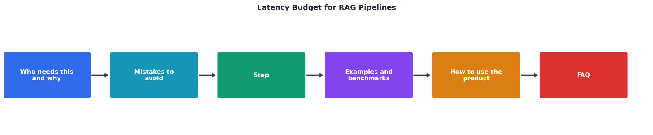
- Define your user-facing SLA. Example: 95% of chat responses complete in 2.5 seconds, 99% in 4 seconds.
- Measure your current baseline. Run 1000 representative queries through your RAG pipeline. Measure each stage. Calculate P50, P95, P99 latencies.
- Allocate budget top-down. Start with your SLA target. Subtract realistic time for each component:
- Embedding: 200 ms (or 50 ms if local).
- Retrieval: 150 ms.
- LLM TTFB: 1000 ms (or less if you can choose a fast provider/region).
- Overhead: 100 ms.
- Remaining buffer: 50 ms (for retries, network jitter).
- Identify the constraint. Which stage consumes the most budget? Usually it is LLM TTFB. Can you reduce it by switching providers, using a faster model, or routing to a closer region?
- Monitor and alert. Set alerts for each stage. When embedding suddenly takes 250 ms (up from 150 ms), you want to know immediately, not after customer complaints.
- Test under load. Your baseline is single-user latency. Under peak traffic, embedding providers, vector stores, and LLM APIs may degrade. Re-run your latency budget with simulated peak traffic.
- Build regional variance into your model selection. If your app serves Tokyo users, do not rely solely on US latency data. Use Observinio or similar to get real regional TTFB numbers before committing to a provider.
Practical Checklist: Latency Budget Setup
Your progress is saved automatically in your browser.
FAQ
Frequently Asked Questions
Monitor Your RAG Latency Budget with Observinio
Latency budgets are only useful if you measure them reliably and across all regions your users occupy. Most monitoring tools focus on your application layer and miss external LLM API variance. Observinio fills this gap: daily synthetic probes from 21 regions measure OpenRouter, OpenAI, and similar endpoints. You get regional TTFB breakdowns, degradation alerts, and a historical trend view. When your Tokyo users start seeing slower responses, you know it within hours, and you have the data to prove whether it is your stack or the provider. Start with your latency budget, then validate it against real-world probe data.
Regional Latency Impact
40–60% variance in response times across regions without monitoring.
Early detection through multi-region probes prevents SLA breaches and user frustration.
Additional Resources
- Removing Latency from RAG Systems: What Actually ... - In production systems, top-3 to top-5 highly relevant chunks consistently outperform large context windows while reducing latency and cost.
- How I Optimized a Production RAG System (and Cut Costs ... - Semantic caching alone cut costs 18% and latency 50% on cache hits. If you're not caching, you're burning money. Hybrid search beats vector-only approaches for latency-sensitive applications.
- Beyond RAG: How cache-augmented generation reduces ... - With Anthropic, you can reduce costs by up to 90% and latency by 85% on the cached parts of your prompt, making cache-augmented generation a critical strategy for global deployments.